
Sometimes when working in Google Sheets, you may want to change your recalculation settings so that formulas refresh either more frequently, or less frequently.
For example, if you are importing financial data and you want your data to refresh so that it is up to date, you may want to update your recalculation settings.In this tutorial, I will show you how to refresh your formulas in Google Sheets.
Changing your Recalculation Settings
Let’s say for example you are using a Google Finance function where you are importing stock prices or some other financial data. The default recalculation settings in Google Sheets is to recalculate “on change” which means every time something changes in the spreadsheet, the formula is recalcualted.
The problem with this is that when importing numbers, the formulas will never recalculate unless you change the settings in Google Sheets.
Here is how to change the recalculation settings:
1. In the top menu select File

2. Then in the drop-down menu select Spreadsheet settings

3. Select the Calculation tab

4. Select the drop-down box below Recalculation. From here you will find the different settings you can apply: on change, on change and every minute, on change and every hour. I have selected “On change and every minute” in this example.

5. Select Save settings when you are done

Now that I have changed the recalculation settings, every single minute my formulas will auto-refresh to pull the most up-to-date data. You can also set it up to only change every hour by selecting the “On change and every hour” option
Closing Thoughts
Changing your recalculation settings in your spreadsheet is a useful thing to know how to do, especially if you regularly work with imported data where the formulas won’t update automatically.
If you do change your recalculation settings, just be cautious about doing this in large files with many formulas. If you have a large spreadsheet with many formulas in it, changing the settings to recalculate more frequently can really slow down your spreadsheet.
It will take much longer for a large spreadsheet to recalculate, so this may not be a good thing to do in some sheets.
How to Configure Auto Refresh for Googlesheets
👉 Follow these steps to create automatically refreshing formulas
In any cell (ie $A$1) type =GOOGLEFINANCE("CURRENCY:USDEUR") which will automatically update (about every 2 minutes)
Using any Cryptosheets custom function, add a reference to that cell at the very end of the formula for the global refresh argument
Syntax =CSPRICE("base","quote","time","exchange","returnType","refresh")
Example 1 =CSPRICE("BTC","USD",,,$A$1)
Example 2 =CSPRICE("BTC","USD",,,GOOGLEFINANCE("CURRENCY:USDEUR"))
Everytime the GoogleFinance cell updates 👉 so will your Cryptosheets data! That's it!

How to Automatically Refresh Cryptosheets Custom Functions Data in Excel & Googlesheets using CS.TIME
Learn how to refresh any Cryptosheets custom function dataset…
👉 Follow these steps to make your Google spreadsheet update automatically at set intervals
Go to File menu
Select Spreadsheet settings
Select Calculation
Adjust the drop down menu to your desired refresh interval
Save your new settings
*Important reminder: you need to add one of the formulas for =NOW() or =TODAY() into your sheet in order for the auto refresh triggers to automatically update your data
There are also a few less official methods that will likely work but may not be as stable:
Use NOW() in any cell. then use that cell as a "dummy" parameter in a function. When NOW() changes every minute the formula recalculates.
Example: =someFunction(a1,b1,c1) * (cell with NOW() / cell with NOW())
Another method is to include a '+ NOW() - NOW()' stunt at the end of the cell formula, with the setting as seen below to recalculate every minute.


How to Refresh Pivot Tables in Google Sheets
Pivot tables are a powerful tool that allows you to summarize data, find patterns and reorganize information. A lot of places of business use them for data analysis in apps like Excel and Google Sheets.
You don’t typically need to refresh data in a pivot table in Google Sheets, as pivot tables typically refresh themselves when the source data is changed. That isn’t always the case, however. Google Sheets might fail to update if you’re working in a large spreadsheet with a lot of data.
If this happens to you, here’s what you’ll need to do to refresh pivot tables in Google Sheets.
How to Refresh Pivot Tables in Google Sheets
One of the easiest ways to refresh a pivot table in Google Sheets is by refreshing the browser you’re using. To do this:Open your pivot table in your browser and make a change, such as filtering a result using the side menu.
Click the Refresh button in your browser window.
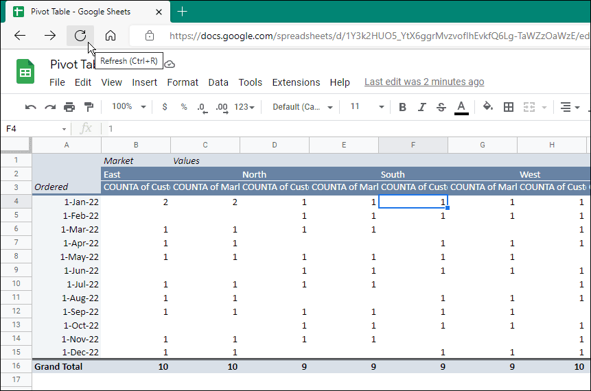
That’s it. Your spreadsheet should update the values you added or removed from the pivot table. The pivot table should dynamically update if you update the data it pulls from the table.
Check Your Data Ranges
Another reason your data may not be appearing correctly in your table is because the data range that your pivot table is pulling data from is incorrect.
If you’ve already added your data, but add a new row of data below it, it won’t show up. Any data rows you add following the creation of the pivot table will not be reflected.
To fix the issue of data not in range in a pivot table, do the following:Click any cell in the pivot table, and the Pivot Table Editor will appear.
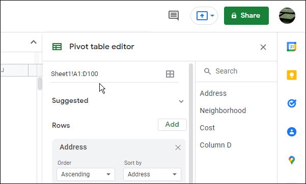
At the top is the pivot table data range—edit the referred data range to add the newly added rows or columns. For example, if the original range was data!B1:E17, you can add a row by updating the range to data!B1:E18.
The table should include the new data and the new row or rows. If it still doesn’t update, refresh your browser as shown in step one.
Check Your Filters
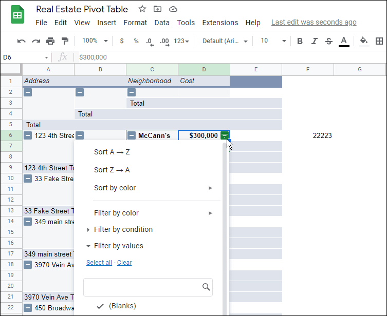
Another reason the pivot table isn’t updating is if you apply a filter, and new items won’t appear. For instance, if you use a filter to a cell or cells in your pivot table, it might hide or display different results.
To fix the filters issue in a Google Sheets pivot table:Open the Pivot Table Editor and scroll to the list of filters.
Click the X symbol next to each one you want to delete—start with the troublesome filters.
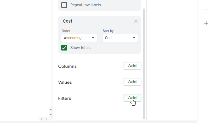
That should fix the problem, and you should start seeing correct values again. To add filters back, bring up the Pivot Table Editor, scroll down to Filters, and create filters by clicking the Add button.
Working With Data in Google Sheets
Now you know how to refresh pivot tables in Google Sheets. Typically, your table in Google Sheets should update dynamically, but if it doesn’t, try refreshing your browser first. If that doesn’t work, try one of the other tips above.
Of course, Google Sheets isn’t the only way to create spreadsheets. For example, if you have Excel, check out how to get the most from pivot tables in the Microsoft app. If you haven’t made one before, read about creating a pivot table in Microsoft Excel.
For Google Sheets, you can create a checklist or insert an image in a Google Sheets spreadsheet. Also, take a look at using Google Sheets to track stocks.


0 Comments